descenso de gradiente usando python y numpy
def gradient(X_norm,y,theta,alpha,m,n,num_it):
    temp=np.array(np.zeros_like(theta,float))
    for i in range(0,num_it):
        h=np.dot(X_norm,theta)
        #temp[j]=theta[j]-(alpha/m)*(  np.sum( (h-y)*X_norm[:,j][np.newaxis,:] )  )
        temp[0]=theta[0]-(alpha/m)*(np.sum(h-y))
        temp[1]=theta[1]-(alpha/m)*(np.sum((h-y)*X_norm[:,1]))
        theta=temp
    return theta


X_norm,mean,std=featureScale(X)
#length of X (number of rows)
m=len(X)
X_norm=np.array([np.ones(m),X_norm])
n,m=np.shape(X_norm)
num_it=1500
alpha=0.01
theta=np.zeros(n,float)[:,np.newaxis]
X_norm=X_norm.transpose()
theta=gradient(X_norm,y,theta,alpha,m,n,num_it)
print theta
Mi theta del código anterior es 100.2 100.2, pero debería ser 100.2 61.09 en matlab, lo cual es correcto.
4 answers
Creo que su código es un poco demasiado complicado y necesita más estructura, porque de lo contrario se perderá en todas las ecuaciones y operaciones. Al final, esta regresión se reduce a cuatro operaciones:
- Calcular la hipótesis h = X * theta
- Calcular la pérdida = h-y y tal vez el costo cuadrado (pérdida^2)/2m
- Calcular el gradiente = X ' * pérdida / m
- Actualizar los parámetros theta = gradiente theta-alfa *
En tu caso, supongo que han confundido m con n. Aquí m indica el número de ejemplos en su conjunto de entrenamiento, no el número de características.
Echemos un vistazo a mi variación de tu código:
import numpy as np
import random

# m denotes the number of examples here, not the number of features
def gradientDescent(x, y, theta, alpha, m, numIterations):
    xTrans = x.transpose()
    for i in range(0, numIterations):
        hypothesis = np.dot(x, theta)
        loss = hypothesis - y
        # avg cost per example (the 2 in 2*m doesn't really matter here.
        # But to be consistent with the gradient, I include it)
        cost = np.sum(loss ** 2) / (2 * m)
        print("Iteration %d | Cost: %f" % (i, cost))
        # avg gradient per example
        gradient = np.dot(xTrans, loss) / m
        # update
        theta = theta - alpha * gradient
    return theta


def genData(numPoints, bias, variance):
    x = np.zeros(shape=(numPoints, 2))
    y = np.zeros(shape=numPoints)
    # basically a straight line
    for i in range(0, numPoints):
        # bias feature
        x[i][0] = 1
        x[i][1] = i
        # our target variable
        y[i] = (i + bias) + random.uniform(0, 1) * variance
    return x, y

# gen 100 points with a bias of 25 and 10 variance as a bit of noise
x, y = genData(100, 25, 10)
m, n = np.shape(x)
numIterations= 100000
alpha = 0.0005
theta = np.ones(n)
theta = gradientDescent(x, y, theta, alpha, m, numIterations)
print(theta)
Al principio creo un pequeño conjunto de datos aleatorios que debería tener este aspecto:
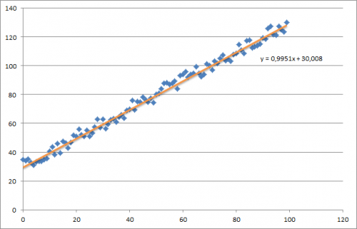
Como puede ver, también agregué la línea de regresión generada y la fórmula que fue calculada por excel.
Debe tener cuidado con la intuición de la regresión utilizando el descenso de gradiente. Como si hace un paso por lotes completo sobre sus datos X, necesita reducir las pérdidas m de cada ejemplo a una sola actualización de peso. En este caso, este es el promedio de la suma sobre los gradientes, por lo tanto la división por m.
Lo siguiente que debe tener cuidado es rastrear la convergencia y ajustar la tasa de aprendizaje. Para el caso, siempre debe realizar un seguimiento de su costo cada iteración, tal vez incluso trazarlo.
Si ejecuta mi ejemplo, el theta devuelto se verá como esto:
Iteration 99997 | Cost: 47883.706462
Iteration 99998 | Cost: 47883.706462
Iteration 99999 | Cost: 47883.706462
[ 29.25567368   1.01108458]
Que en realidad está bastante cerca de la ecuación que fue calculada por excel (y = x + 30). Tenga en cuenta que a medida que pasamos el sesgo en la primera columna, el primer valor theta denota el peso del sesgo.
Warning: date(): Invalid date.timezone value 'Europe/Kyiv', we selected the timezone 'UTC' for now. in /var/www/agent_stack/data/www/ajaxhispano.com/template/agent.layouts/content.php on line 61
2013-12-21 12:22:58
A continuación puede encontrar mi implementación de descenso de gradiente para el problema de regresión lineal.
Al principio, calculas el gradiente como X.T * (X * w - y) / N y actualizas tu theta actual con este gradiente simultáneamente.
- X: matriz de características
- y: valores objetivo
- w: pesos / valores
- N: tamaño del conjunto de entrenamiento
Aquí está el código python:
import pandas as pd
import numpy as np
from matplotlib import pyplot as plt
import random
def generateSample(N, variance=100):
X = np.matrix(range(N)).T + 1
Y = np.matrix([random.random() * variance + i * 10 + 900 for i in range(len(X))]).T
return X, Y
def fitModel_gradient(x, y):
N = len(x)
w = np.zeros((x.shape[1], 1))
eta = 0.0001
maxIteration = 100000
for i in range(maxIteration):
error = x * w - y
gradient = x.T * error / N
w = w - eta * gradient
return w
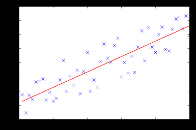
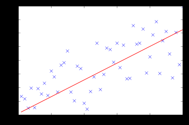
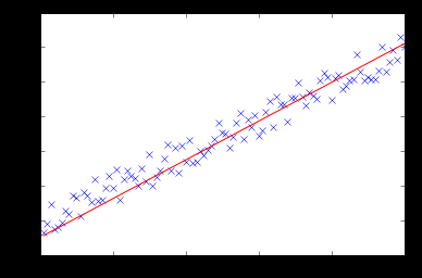
def plotModel(x, y, w):
plt.plot(x[:,1], y, "x")
plt.plot(x[:,1], x * w, "r-")
plt.show()
def test(N, variance, modelFunction):
X, Y = generateSample(N, variance)
X = np.hstack([np.matrix(np.ones(len(X))).T, X])
w = modelFunction(X, Y)
plotModel(X, Y, w)
test(50, 600, fitModel_gradient)
test(50, 1000, fitModel_gradient)
test(100, 200, fitModel_gradient)
Warning: date(): Invalid date.timezone value 'Europe/Kyiv', we selected the timezone 'UTC' for now. in /var/www/agent_stack/data/www/ajaxhispano.com/template/agent.layouts/content.php on line 61
2016-04-03 19:22:22
Sé que esta pregunta ya ha sido contestada pero he hecho alguna actualización a la función GD :
  ### COST FUNCTION

def cost(theta,X,y):
     ### Evaluate half MSE (Mean square error)
     m = len(y)
     error = np.dot(X,theta) - y
     J = np.sum(error ** 2)/(2*m)
     return J

 cost(theta,X,y)


def GD(X,y,theta,alpha):

    cost_histo = [0]
    theta_histo = [0]

    # an arbitrary gradient, to pass the initial while() check
    delta = [np.repeat(1,len(X))]
    # Initial theta
    old_cost = cost(theta,X,y)

    while (np.max(np.abs(delta)) > 1e-6):
        error = np.dot(X,theta) - y
        delta = np.dot(np.transpose(X),error)/len(y)
        trial_theta = theta - alpha * delta
        trial_cost = cost(trial_theta,X,y)
        while (trial_cost >= old_cost):
            trial_theta = (theta +trial_theta)/2
            trial_cost = cost(trial_theta,X,y)
            cost_histo = cost_histo + trial_cost
            theta_histo = theta_histo +  trial_theta
        old_cost = trial_cost
        theta = trial_theta
    Intercept = theta[0]
    Slope = theta[1]
    return [Intercept,Slope]

res = GD(X,y,theta,alpha)
Esta función reduce el alfa sobre la iteración haciendo que la función también converja más rápido ver Estimación de regresión lineal con Descenso de Gradiente (Descenso más pronunciado) para un ejemplo en R. I aplicar la misma lógica pero en Python.
Warning: date(): Invalid date.timezone value 'Europe/Kyiv', we selected the timezone 'UTC' for now. in /var/www/agent_stack/data/www/ajaxhispano.com/template/agent.layouts/content.php on line 61
2018-03-21 05:12:01
Siguiendo la implementación de @thomas-jungblut en python, hice lo mismo para Octave. Si encuentra algo mal, por favor hágamelo saber y arreglaré + actualizar.
Los datos provienen de un archivo txt con las siguientes filas:
1 10 1000
2 20 2500
3 25 3500
4 40 5500
5 60 6200
Piense en ello como una muestra muy aproximada de las características [número de dormitorios] [mts2] y la última columna [precio del alquiler] que es lo que queremos predecir.
Aquí está la implementación de Octava:
%
% Linear Regression with multiple variables
%

% Alpha for learning curve
alphaNum = 0.0005;

% Number of features
n = 2;

% Number of iterations for Gradient Descent algorithm
iterations = 10000

%%%%%%%%%%%%%%%%%%%%%%%%%%%%%%%%%%%%%%%%%%
% No need to update after here
%%%%%%%%%%%%%%%%%%%%%%%%%%%%%%%%%%%%%%%%%%

DATA = load('CHANGE_WITH_DATA_FILE_PATH');

% Initial theta values
theta = ones(n + 1, 1);

% Number of training samples
m = length(DATA(:, 1));

% X with one mor column (x0 filled with '1's)
X = ones(m, 1);
for i = 1:n
  X = [X, DATA(:,i)];
endfor

% Expected data must go always in the last column
y = DATA(:, n + 1)

function gradientDescent(x, y, theta, alphaNum, iterations)
  iterations = [];
  costs = [];

  m = length(y);

  for iteration = 1:10000
    hypothesis = x * theta;

    loss = hypothesis - y;

    % J(theta)
    cost = sum(loss.^2) / (2 * m);

    % Save for the graphic to see if the algorithm did work
    iterations = [iterations, iteration];
    costs = [costs, cost];

    gradient = (x' * loss) / m; % /m is for the average

    theta = theta - (alphaNum * gradient);
  endfor

  % Show final theta values
  display(theta)

  % Show J(theta) graphic evolution to check it worked, tendency must be zero
  plot(iterations, costs);

endfunction

% Execute gradient descent
gradientDescent(X, y, theta, alphaNum, iterations);
Warning: date(): Invalid date.timezone value 'Europe/Kyiv', we selected the timezone 'UTC' for now. in /var/www/agent_stack/data/www/ajaxhispano.com/template/agent.layouts/content.php on line 61
2018-04-03 02:01:06